A Practical Guide to Converting, Importing, and Exporting Geospatial Data with GDAL’s ogr2ogr Tool
Intro
Geospatial data is essential in numerous fields, from urban planning and environmental monitoring to navigation systems, disaster management and safety.
Over the years, various file formats have been developed to store and share geographic information, each with its own set of features and use cases. Common geospatial file formats include Shapefile, KML, GPX, GeoPackage and GeoJSON, which differ in their structure, flexibility, and compatibility with different software tools.
For developers, GIS analysts, and data scientists working with geospatial data, the ability to efficiently manage and manipulate these files is crucial. One of the most powerful ways to work with geospatial data is by importing it into a PostGIS database, a spatial extension of PostgreSQL. PostGIS provides robust capabilities for spatial queries, analysis, and storage, making it a popular choice for managing large-scale geospatial datasets.
However, converting between different geospatial file formats and importing them into PostGIS can be a complex task. Fortunately, the ogr2ogr library, part of the GDAL (Geospatial Data Abstraction Library) suite, offers a straightforward and powerful solution. This command-line tool allows users to convert between a wide variety of geospatial file formats, while also enabling seamless integration with PostGIS for efficient data import and export.
NOTE: There is also the python wrapper around the GDAL library. However, sometimes it’s more convenient to use a command line tool, rather than taking care of a Python environment just to import data.
Article Overview
This article provides a comprehensive guide on handling various geospatial file formats and importing them into a PostGIS database using the powerful ogr2ogr tool from the GDAL suite. It covers common formats like Shapefile, KML, GPX, GeoPackage and GeoJSON, outlining their strengths, limitations, and ideal use cases.
A practical walkthrough is given for:
- Extracting building and street data from OpenStreetMap using the Overpass Turbo API.
- Converting formats (e.g., KML to Shapefile and GeoPackage) while highlighting quirks like Shapefile’s field length and type limitations.
- Importing to PostGIS using Docker and
ogr2ogr, with tips like promoting geometries to multi-polygons and speeding up imports usingPG_USE_COPY=YES. - Exporting from PostGIS to formats like CSV and Excel for downstream use.
As example data we use the OSM buildings and streets data pulled from OpenStreeMap OSM via the overpass turbo API.
NOTE: For this specific use case - OSM data to PostGIS - we could have used the dedicated
osm2pgsqlcommandline tool, but we want to keep things more flexible for this article.
Geospatial Data File Formats
A quick intro to the most common ones and their advantages and limitations.
GeoPackage (.gpkg)
The GeoPackage (GPKG) format is a modern, efficient, and standards-based format for storing geospatial data. It is based on SQLite, meaning it is a single-file database that can store multiple layers of vector and raster data, as well as metadata, indexes, and styles.
Multiple layers could be a vector layer with points representing major cities and their attributes (e.g., population, country), a polygon layer representing country boundaries and a raster layer containing satellite imagery.
Advantages:
- Single File: Unlike Shapefiles, which require multiple files, GeoPackage stores everything in one
.gpkgfile. - Supports Multiple Layers: Can store vector, raster, and metadata in the same file.
- Efficient & Compact: Uses SQLite compression and indexing for optimised performance.
- No Field Name Limits: Unlike Shapefiles, GeoPackage supports long attribute field names.
- Cross-Platform & Open Standard: Compatible with many GIS applications like QGIS, GDAL, and ArcGIS.
Limitations:
- Software Support: While widely supported, some legacy GIS tools may not fully support all GeoPackage features.
- File Corruption Risk: Since it’s a database file, improper handling (e.g., unexpected shutdowns) can lead to corruption.
Shapefile (.shp)
The Shapefile format is one of the most widely used formats in Geographic Information Systems (GIS) for storing geographic data such as points, lines, and polygons.
A Shapefile typically consists of several files:
.shp: The file stores geometric data (shapes).shx: The shape index for faster retrieval.dbf: Attribute data in tabular format (e.g., names, population)
Limitations:
- File Size: Shapefiles can become quite large, especially for complex data, but .shp and .dbf component files cannot exceed 2 GB (approx. 70 Mio. points see wikipedia)
- Limited Data Types: Shapefiles are mostly used for simple geometry (points, lines, and polygons), don’t support advanced data structures like nested geometries and cannot mix polygon, line and point data in one file. Buildings (polygons), addresses (points) and streets (lines) would need to be stored in three separate datasets. This can also be an advantage at times, since you know what you get.
- No Support for Advanced Attributes: Unlike more modern formats like GeoJSON, Shapefiles don’t support complex nested attributes or metadata. The maximum number of fields is 255 and supported field types are: floating point, integer, date (no time storage), and text (maximum 254 character). Floating point numbers may contain rounding errors since they are stored as text.
- Field name length: they do not allow field names longer than 10 characters
For more in depth considerations see for example here.
KML (Keyhole Markup Language)
KML is an XML-based format used to represent geographic data for applications like Google Earth and Google Maps.
It’s simple to read and allows for the representation of places, routes, and polygons, along with advanced features like 3D models and image overlays. You’ll often come across zipped KML files: KMZ files with a .kmz extension.
A KML file representing the Colosseum’s location using latitude and longitude coordinates might look like this:
<kml xmlns="http://www.opengis.net/kml/2.2">
  <Document>
    <Placemark>
      <name>Colosseum</name>
      <Point>
        <coordinates>12.4924,41.8902,0</coordinates>
      </Point>
    </Placemark>
  </Document>
</kml>
Limitations:
- File Size: KML files can become cumbersome when dealing with large datasets.
- Performance Issues: As the number of features increases, KML files can slow down the rendering in applications like Google Earth or Maps.
- Limited to Simple Geometries: KML doesn’t support advanced geometries or types of spatial analysis as robustly as formats like Shapefile or GeoJSON.
GeoJSON (.geojson)
GeoJSON is a format based on JSON (JavaScript Object Notation) used for encoding geographic data structures.
It is widely used for web-based mapping applications, especially when working with JavaScript libraries like Leaflet and Mapbox.
A GeoJSON file with the coordinates outlining Amsterdam’s boundary might look like this:
{
  "type": "FeatureCollection",
  "features": [
    {
      "type": "Feature",
      "geometry": {
        "type": "Polygon",
        "coordinates": [
          [
            [4.9041, 52.3676],
            [4.9141, 52.3676],
            [4.9141, 52.3776],
            [4.9041, 52.3776],
            [4.9041, 52.3676]
          ]
        ]
      },
      "properties": {
        "name": "Amsterdam",
        "country": "Netherlands",
        "population": "872,680"
      }
    }
  ]
}
Limitations:
- File Size: While GeoJSON is text-based and human-readable, it can become large for complex datasets.
- Limited Support for Advanced Geometries: GeoJSON supports basic shapes like points, lines, and polygons, but more complex geometries or 3D data aren’t well-supported.
- Not Ideal for Large-Scale Data: GeoJSON is generally not optimized for handling extremely large datasets (e.g., national-level datasets).
GPX (GPS Exchange Format)
GPX is a lightweight XML-based format used for storing GPS data such as tracks, routes, and waypoints. It’s commonly used for activities like hiking, biking, and geocaching. GPX files are easy to create and share across different GPS devices and mapping software.
A GPX file tracking a route might look like this:
<?xml version="1.0" encoding="UTF-8"?>
<gpx version="1.1" creator="GPX Creator">
  <trk>
    <name>Chamonix Hiking Trail</name>
    <trkseg>
      <trkpt lat="45.9237" lon="6.8694">
        <ele>1035</ele>
        <time>2025-03-25T08:00:00Z</time>
      </trkpt>
      <trkpt lat="45.9325" lon="6.8751">
        <ele>1075</ele>
        <time>2025-03-25T08:15:00Z</time>
      </trkpt>
    </trkseg>
  </trk>
</gpx>
Tracking a hiker in The Alps, near Chamonix, with waypoints representing specific locations on the hiking trail.
Limitations:
- No Support for Complex Geometry: GPX is focused on simple points, routes, and tracks, and lacks support for complex shapes or multi-layered data.
- Limited Metadata: GPX files are simple and don’t support complex attributes or detailed metadata.
- Not Ideal for Large Datasets: GPX isn’t designed for large amounts of data, such as a full city map or extensive geographic dataset.
Summary of Limitations:
Each format has its strengths and weaknesses, and the choice of which one to use depends on the specific needs of your project, such as the type of data you’re working with and the software or platform you’re using.
- Shapefile: Large file sizes, multiple required files, and no support for advanced attributes.
- KML: Performance issues with large datasets and limited support for complex geometries.
- GPX: Lacks support for complex geometries and metadata, and is not ideal for large datasets.
- GeoJSON: Can become large for complex datasets and has limited support for advanced geometries.
- GeoPackage: Requires software that supports SQLite-based geospatial data and has a risk of file corruption if not handled properly.
Getting OSM data
To have some example data to work with we pull streets and buildings data from OpenStreetMaps using the Overpass turbo UI with the following Overpass QL query for buildings:
[out:json][timeout:3000];(
way["building"](52.495,-0.376,52.664,-0.059);
relation["building"]["type"="multipolygon"](52.495,-0.376,52.664,-0.059);
);out;>;out qt;
We then click on export and download the .kml and .geojson files.
For street data we used:
[out:json][timeout:3000];(
  way["highway"](52.495,-0.376,52.664,-0.059);
  way["highway"="footway"](52.495,-0.376,52.664,-0.059);
);out;>;out qt;
and downloaded the .gpx file.
The bounding box (52.495,-0.376,52.664,-0.059) is the area around Perterborough, UK:
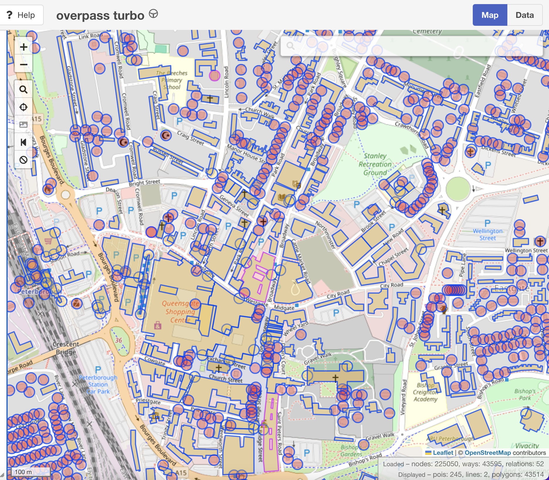 A zoomed-in look into the buildings data
NOTE: We could have downloaded the data via
curlor python requests instead of using the Overpass turbo UI. For more on how to download and work with OSM data see OpenStreetMap Data article.
Folder Structure
Now we should have buildings data as .kml and .geojson files, and streets in .gpx format:
data/raw/buildings.geojson: Contains building data in GeoJSON format.data/raw/buildings.kml: Contains building data in KML format.data/raw/streets.gpx: Contains street data in GPX format.
Conversions
In order to show more formats and demonstrate conversions from one format to another, we will transform the .kml file to a shapefile and a geopackage.
Kml to Shapefile
Since a shapefile consists of several files (.dbf, .prj, .shp, .shx see above), we’ll add a directory and place the target shapefile in it to keep track of them.
Running the command without any arguments other than target and source file:
mkdir -p buildings
ogr2ogr -f 'ESRI Shapefile' buildings/buildings.shp buildings.kml
will lead to warnings for fields with field name character length above 10:
Warning 6: Normalized/laundered field name: 'contact_website' to 'contact_we'
Warning 6: Normalized/laundered field name: 'opening_hours' to 'opening_ho'
Warning 6: Normalized/laundered field name: 'payment_american_express' to 'payment_am'
as well as the file having more than 255 number of fields:
Warning 1: Creating a 256th field, but some DBF readers might only support 255 fieldsWe also get actual errors:
ERROR 1: Attempt to write non-polygon (LINESTRING) geometry to POLYGON type shapefile.
ERROR 1: Attempt to write non-polygon (POINT) geometry to POLYGON type shapefile.
Since shapefiles only support ONE geometry type per dataset we filter the polygons from the .kml with the -nlt argument.
ogr2ogr -f 'ESRI Shapefile' \
buildings/buildings.shp buildings.kml \
-nlt POLYGON \
-overwrite \
-skipfailures
Because of this limitation the OSM data we pulled would need to be stored in three separate .shp files/folders and be written to PostGIS in three separate ogr2ogr commands - one for each geometry type, for example: one with --overwrite argument to re-initialise the table and two subsequent --append commands.
KML to Geopackage
Converting from kml to GeoPackage is more straightforward:
ogr2ogr -f 'GPKG' buildings.gpkg buildings.kmlNow we can connect to buildings.gpkg as if it were a SQLite database via sqlite3 command-line tool:
sqlite3 data/raw/buildings.gpkgand search, for example, the tables and indexes in the .gpkg file:
sqlite> .tables
gpkg_contents
gpkg_extensions
gpkg_geometry_columns
gpkg_ogr_contents
gpkg_spatial_ref_sys
gpkg_tile_matrix
gpkg_tile_matrix_set
overpass-turbo.eu export
rtree_overpass-turbo.eu export_geom
rtree_overpass-turbo.eu export_geom_node
rtree_overpass-turbo.eu export_geom_parent
rtree_overpass-turbo.eu export_geom_rowid
The gpkg_contents table holds
- the actual name of the user-defined data tables (
table_name) - the
data_type(e.g. “tiles”, “features”, “attributes”), - the spatial extents of the content (
min_x, min_y, max_x, max_y) - spatial reference system
srs_id.
In our example:
| table_name | data_type | identifier | description | last_change | min_x | min_y | max_x | max_y | srs_id |
|---|---|---|---|---|---|---|---|---|---|
| overpass-turbo.eu export | features | overpass-turbo.eu export | 2025-03-27T15:17:35.254Z | -0.3742458 | 52.495 | -0.058 | 52.664 | 4326 |
You can also connect to the file via any DB tool and explore the data directly. For example you can query the overpass-turbo.eu export table with DBeaver and see the attributes and the spatial data:
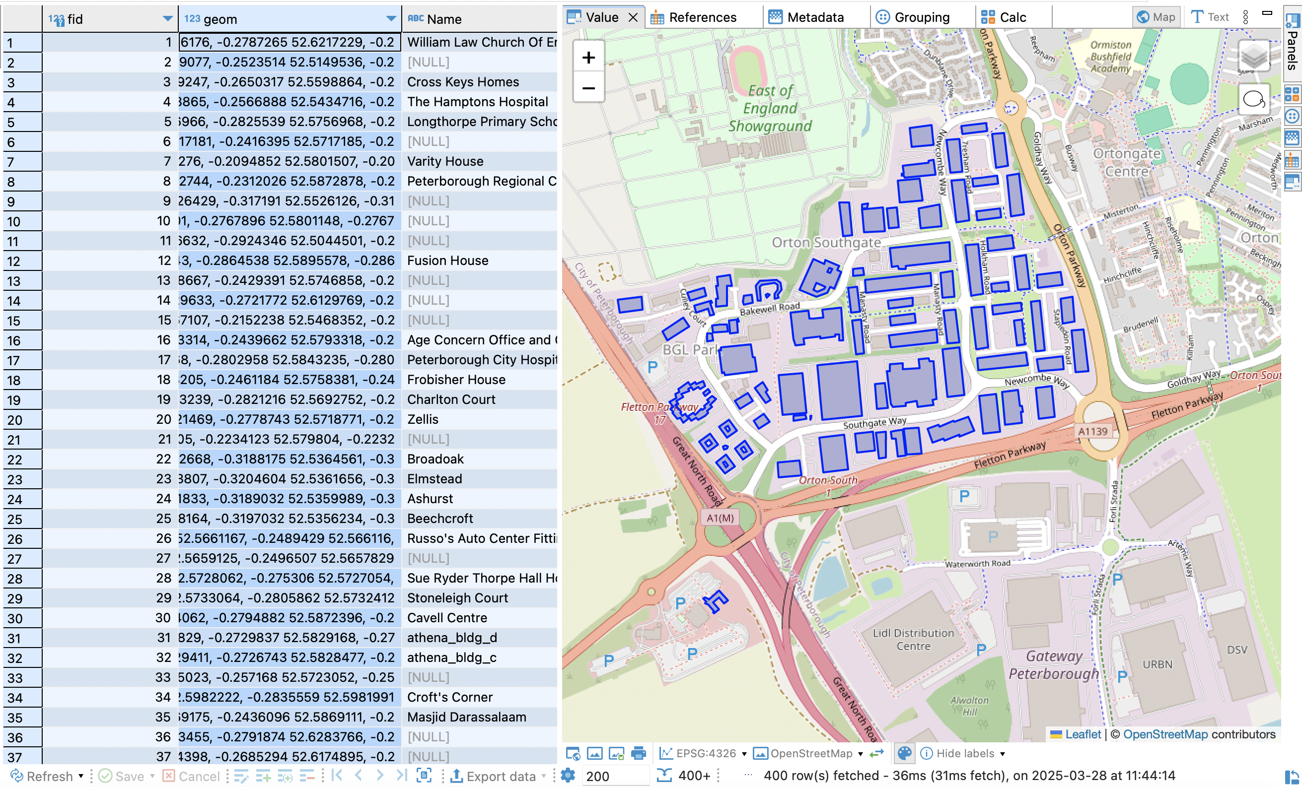 Geopackage file viewed through DBeaver
File Sizes
Here are the file sizes of four different formats: .kml, Shapefile, GeoJson and GeoPackage. The shapefile is orders of magnitude bigger than the others:
| Size | File |
|---|---|
| 1.1G | buildings (shapefile folder) |
| 35M | buildings.geojson |
| 27M | buildings.gpkg |
| 19M | buildings.kml |
a closer look into the Shapefile folder
| Size | File |
|---|---|
| 1.1G | buildings.dbf |
| 6.7M | buildings.shp |
| 340K | buildings.shx |
| 145 | buildings.prj |
reveals the attributes file .dbf is the culprit with over 1GB.
This makes sense. OSM data is very sparse with many different attributes rarely populated, resulting in a lot of (mostly empty) columns in the .dbf file. For OSM data a key-value based format like geojson and .kml is more efficient.
Write to DB
It is time to walk through the imports to PostGIS. We use docker-compose to run PostGIS (postgis/postgis:latest) and a client with the GDAL library installed based on the ghcr.io/osgeo/gdal:ubuntu-full-latest image. See geospatial stack a quick tutorial for setting up PostGIS with a GDAL client.
KML to PostGIS
To import a .kml file to PostGIS all we need are
- the Postgres user, host, database name and password,
- the name of the KML file
and we can specify a wide array of options, such as
- the name of the target table,
- whether we want to append or overwrite the table,
- the geometry column name,
- the spatial reference system (not set here)
and many more. Here is an example:
ogr2ogr -f "PostgreSQL" \
    PG:"host=$PGHOST user=$POSTGRES_USER dbname=$POSTGRES_DB password=$POSTGRES_PASSWORD" \
    "./data/raw/buildings.kml" \
    -nln "osm_buildings_kml" `# Set target table name` \
    -overwrite   `# Overwrite existing table` \
    -lco GEOMETRY_NAME=geom   `# Set geometry column name`\
    -lco FID=gid   `# Set feature ID column name`\
    -lco PRECISION=NO   `# Disable numeric precision` \
    -progress   `# Enable progress reporting` \
    -skipfailures  `# Skip features that fail to convert`
Shapefile to PostGIS
If you use the same command as above to import the shapefile just by replacing file and table names you’ll get the following error:
ERROR 1: COPY statement failed.
ERROR:  Geometry type (MultiPolygon) does not match column type (Polygon)
PostGIS only expected POLYGONs and complained when it saw a MULTIPOLYGON.
We can pass the -nlt PROMOTE_TO_MULTI command to instruct ogr2ogr to make all polygons multi-polygons.
ogr2ogr -f "PostgreSQL" \
    PG:"host=$PGHOST user=$POSTGRES_USER dbname=$POSTGRES_DB password=$POSTGRES_PASSWORD" \
    "/data/raw/buildings/buildings.shp" \
    -nln "osm_buildings_shp" \
    -nlt PROMOTE_TO_MULTI \
    -overwrite \
    -lco GEOMETRY_NAME=geom \
    -lco FID=gid \
    -lco PRECISION=NO \
    -progress \
    -skipfailures
In fact if we look at the geometry types in the target table osm_buildings_shp:
select
  st_geometrytype(geom),
  count(*)
from
  osm_buildings_shp
group by 1| st_geometrytype | count |
|---|---|
| ST_MultiPolygon | 43484 |
All polygons got promoted (regardless of being single or multi), but we got all into PostGIS.
Geojson and Geopackage to PostGIS
For these we only replace the filename and target table name of the KML command above. The only difference between the resulting tables are the column names, because they are different in the original data files.
For example the OSM geojson stores address fields as addr:city, addr:country, addr:postcode, addr:suburb, whereas the KML from which we created the Geopackage has the field names already cleaned: addr_city, addr_country, addr_postcode, addr_suburb.
GPX
We dowloaded the street data in the .gpx format. GPX can store data in different feature types. The ogrinfo command can help look into the file:
ogrinfo -so streets.gpxINFO: Open of `streets.gpx'
using driver `GPX' successful.
1: waypoints (Point)
2: routes (Line String)
3: tracks (Multi Line String)
4: route_points (Point)
5: track_points (Point)
For more details sew the ogr2ogr documentation for gpx.
The following command will pick tracks using the -sql argument of the ogr2ogr command and import them to table osm_streets in PostGIS:
ogr2ogr -f "PostgreSQL" \
    PG:"host=$PGHOST user=$POSTGRES_USER dbname=$POSTGRES_DB password=$POSTGRES_PASSWORD" \
    "data/raw/streets.gpx" \
    -nln "osm_streets"\
    -sql "Select * From tracks"  `# Select only the tracks from the gpx file`\
    -overwrite\
    -lco GEOMETRY_NAME=geom \
    -lco FID=gid \
    -lco PRECISION=NO
Loading Times
A quick comparison of loading times.
For streets data the GPX file loaded 24,733 multi-linestrings and attributes in 30 seconds. For the same buildings data the import times don’t vary much between formats:
| File Format | Loading Time (seconds) |
|---|---|
| GeoJSON | 96 |
| GeoPackage | 97 |
| KML | 100 |
| Shapefile | 104 |
| However, they are all pretty slow considering we are importing only around 40,000 geometries. |
Adding PG_USE_COPY=YES to the config argument speeds up writing to PostGIS significantly:
ogr2ogr -f "PostgreSQL" \
    PG:"host=$PGHOST user=$POSTGRES_USER dbname=$POSTGRES_DB password=$POSTGRES_PASSWORD" \
    "./data/raw/buildings.kml" \
    -nln "osm_buildings_kml" `# Set target table name` \
    -overwrite   `# Overwrite existing table` \
    -lco GEOMETRY_NAME=geom   `# Set geometry column name`\
    -lco FID=gid   `# Set feature ID column name`\
    -lco PRECISION=NO   `# Disable numeric precision` \
    -progress   `# Enable progress reporting` \
    -skipfailures  `# Skip features that fail to convert` \
    --config PG_USE_COPY=YES
30x speedup: Using PG_USE_COPY=YES in the PostGIS database import command reduces import time for the .kml file 100s down to 3 seconds.
From the number of different geometry types we can see which formats have similar behaviour:
| ST_LineString | ST_MultiPolygon | ST_Point | ST_Polygon | |
|---|---|---|---|---|
| osm_buildings_geojson | 2 | 11 | 245 | 43471 |
| osm_buildings_gpkg | 2 | 11 | 245 | 43471 |
| osm_buildings_kml | 2 | 11 | 245 | 43471 |
| osm_buildings_shp | nan | nan | nan | 43474 |
.geojson, .kml and .gpkg lead to the same number of geometry types. Because of the strict type handling of .shp files, we essentially only kept polygons.
Indexes
When importing via ogr2ogr you don’t have to worry about indexing the geometry, it’s done for you.
- The FID column is added as a primary key
- The geometry is indexed with a
GISTindex
Exporting from PostGIS
Now for the last part: exporting data from PostGIS to commonly used formats.
From PostGIS to csv
Here we use ogr2ogr’s CSV driver to download data:
ogr2ogr -f "CSV" \
    "buildings.csv" \
    PG:"host=$PGHOST user=$POSTGRES_USER dbname=$POSTGRES_DB password=$POSTGRES_PASSWORD" \
    -sql "SELECT  _id, name, building, addr_city, addr_postcode, geom FROM osm_buildings_kml" \
    -lco GEOMETRY=AS_WKT `# transform geometry to WKT representation` \
    -lco GEOMETRY_NAME=geom `# the column name of the WKT (defaults to WKT if not specified)` \
    -progress \
-skipfailures - The
-sqlarguments lets you select the columns - The
-lcoarguments let you set the name of the geometry and request it as well-known-text (WKT) format
Here are the first two rows of buildings.csv file:
geom,_id,name,building,addr_city,addr_postcode
"POLYGON ((-0.278 52.6216,...,-0.278 52.621))",relation/1303438,William Law Church Of England Primary School,school,Peterborough,PE4 5DT
"POLYGON ((-0.252 52.514,...,-0.252 52.514))",relation/1303959,,yes,,
From PostGIS to Excel
If for some crazy reason you need to export to excel with geometries you’ll be disappointed: no geometry support is available directly for excel. However-as for CSVs above-you can get the WKT representation of the geometries via the SQL command.
ogr2ogr -f "XLSX" \
"buildings.xlsx" \
PG:"host=$PGHOST user=$POSTGRES_USER dbname=$POSTGRES_DB password=$POSTGRES_PASSWORD" \
-sql "SELECT _id, name, building, addr_city, addr_postcode, st_astext(geom) geom FROM osm_buildings_kml" \
-nln "osm_buildings" `# the sheet name` \
-progress \
-skipfailures 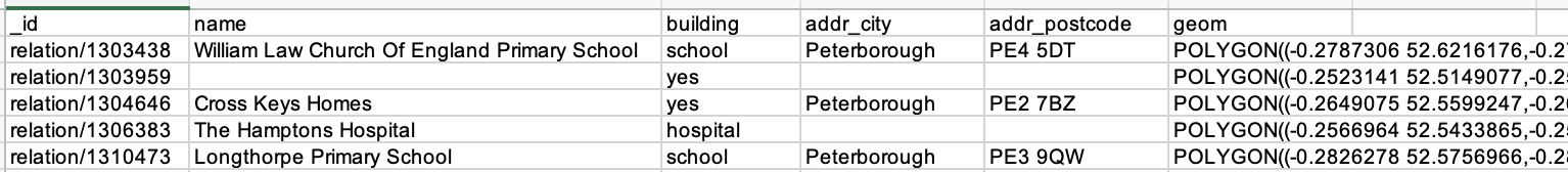 OSM data extracted from PostGIS to buildings.xlsx excel with WKT geometries
Conclusion
Working with geospatial data often involves navigating a variety of file formats, each with its own strengths and limitations. Understanding these differences is essential for selecting the right format for storage, conversion, and analysis.
Whether you’re dealing with compact and modern formats like GeoPackage, web-friendly options like GeoJSON, or legacy standards like Shapefile, having the ability to efficiently transform and load this data into a robust system like PostGIS is a key skill for any GIS professional or data scientist.
We demonstrated how to obtain OpenStreetMap data, explore different formats, and use ogr2ogr to convert between them and import them into PostGIS. We also highlighted critical considerations like field name truncation in Shapefiles, performance boosts with PG_USE_COPY=YES, and the importance of geometry type consistency.
By using tools like ogr2ogr and PostGIS, you can streamline your geospatial workflows, handle large and complex datasets, and prepare your spatial data for deeper analysis.
No matter your stack—command-line, database, or Python, knowing how to bridge the gap between formats and databases ensures you’re ready to tackle any geospatial challenge.