PostGIS DBSCAN Tutorial: Cluster Building Polygons with SQL, Not Code
Looking to cluster building footprints or other non-point geometries directly in your PostGIS database? This tutorial shows how to use the ST_ClusterDBSCAN function to run DBSCAN clustering in SQL—without exporting to Python or GIS tools.
We’ll compare PostGIS results with Python’s scikit-learn DBSCAN, using OpenStreetMap building data and different geometry-based distance strategies. Whether you’re working on spatial analytics, urban planning, or GIS automation, this guide helps you choose the right DBSCAN approach for your geospatial datasets.
Intro
In our previous article DBSCAN general we explored how DBSCAN works and compared its implementation across tools like Python, Julia, R, and SQL. We found that PostGIS’s ST_ClusterDBSCAN stands out for clustering non-point geometries efficiently and directly within the database — no exports or external environments required.
In this follow-up, we show how to use ST_ClusterDBSCAN for clustering real-world spatial data, such as building polygons from OpenStreetMap. Unlike point-based clustering, these geometries often require true shape-to-shape distance calculations. In some cases, only touching buildings should be considered neighbours — making epsilon=0 a practical setting. We’ll walk through a full example to demonstrate how this works in practice.
PostGIS DBSCAN query
If you want to code along we recommend following our geospatial setup quickstart and importing some OpenStreetMap data (REF TO IMPORT OSM DATA).
We’ve imported OSM building polygons into a PostGIS DB.
The geometry column geom is in the geographic 4326 coordinate reference system (CRS) (EPSG:4326 also known as WGS 84, a common geographic CRS using latitude/longitude). To have a better understanding of distances when picking epsilon for DBSCAN we need our coordinates in a flat projection CRS. Since our data is in the UK, we’ll transform our geometries to the UK grid EPSG:27700, in the unit of metres, before clustering.
The following SQL query is all we need to get DBSCAN cluster labels:
SELECT
*,
ST_ClusterDBSCAN(
st_transform(geom, 27700), -- transform into a crs where units are metres so our epsilon is easier to pick
eps := 20,
minpoints := 2
) OVER () as cluster_id
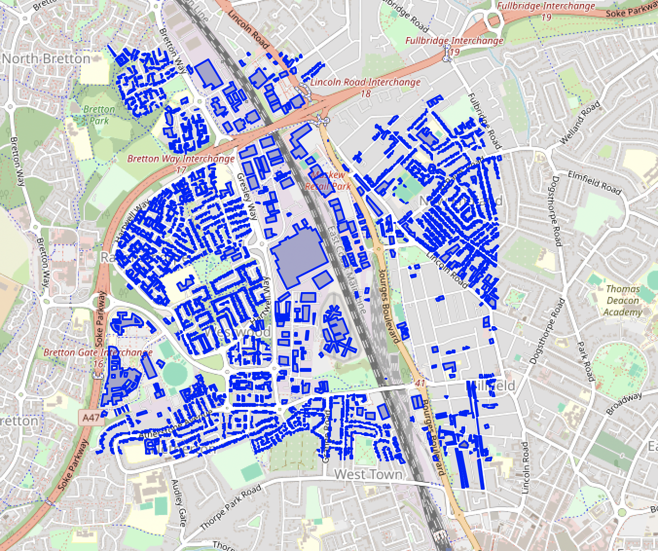
FROM osm_buildings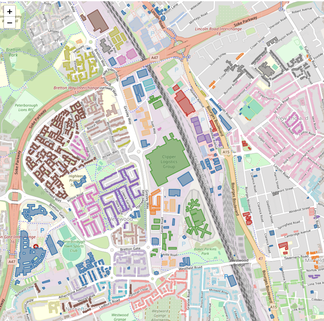 Colour-coded PostGIS DBSCAN clusters
Comparison with Sklearn DBSCAN
We willl now try to reproduce the same results we obtained in PostGIS via Python’s Sklearn DBSCAN using a precomputed distance matrix.
Using distance matrix
from scipy.sparse import csr_array
import geopandas as gpd
from sqlalchemy import create_engine
# db connection
engine = create_engine(f"postgresql+psycopg2://{pg_user}:{pg_pw}@{host}:{port}/{pg_db}")

# pull data from postgis into a geopandas dataframe
df = gpd.read_postgis("select * from osm_buildings" ,con=engine, geom_col="geom")

# get the pairwise distances between the buildings to uk grid
geoms_2d = df[["geom"]].to_crs(27700)

# add 200m buffer to get the neighbours
neighbors = geoms_2d.sjoin(geoms_2d.buffer(200).to_frame())

# merge the results with the original data to get the geometry
neighbors = neighbors.merge(geoms_2d, left_on="index_right", right_index=True)

# calculate the distance between the two geometries
neighbors["distance"] = neighbors["geom_x"].distance(neighbors["geom_y"])
neighbors = neighbors.reset_index()

# make sparse array
neighbors_sparse = csr_array((neighbors['distance'], (neighbors['index'], neighbors['index_right'])))

# and cluster
from sklearn.cluster import DBSCAN
dbscan = DBSCAN(eps=eps, min_samples=min_samples, metric="precomputed")
clusters = dbscan.fit_predict(neighbors_sqarse)
We can compare the resulting clusters with the ones we obtained from PostGIS by looking at various cluster performance evaluation metrics using the PostGIS clusters as the ground truth. The clusters using pairwise distance matrix in Sklearn are identical!:
{
	'Homogeneity': 1.0,
	'Completeness': 1.0,
	'V-measure': 1.0,
	'Adjusted Rand Index': 1.0,
	'Adjusted Mutual Information': 1.0
}
Using points from polygons plus extra radius
Calculating and passing the precomputed distance matrix can be time-consuming and add complexity.
We can simplify the polygons to circles by clustering the xs and ys of the points and adding an extra length to epsilon, representing a radius.
This radius should be a good characteristic length for all buildings.
We can try a few, with the area of the building :
- char_len_circle: Radius of a circle with the same area as building
- char_len_square: Half of a square’s side with the same area as the building
- minimum_bounding_radius: Radius of the smallest circle that contains the building geometry
- maximum_inscribed_radius: Largest radius of a circle that can be inscribed within the building
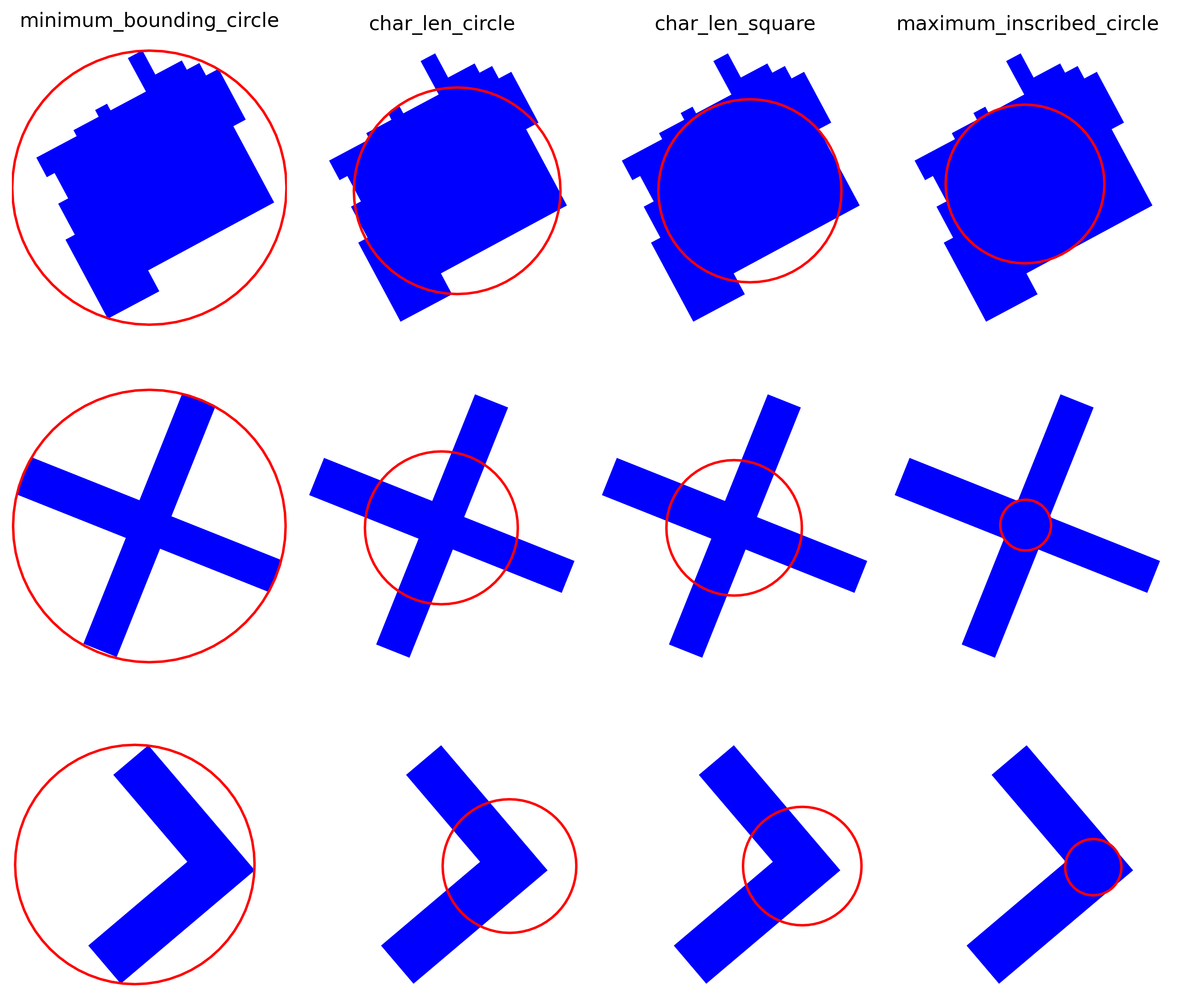 Minimum bounding radius, characteristic length (circle, square) and maximum inscribed radius of a few buildings. None can cover all building shapes perfectly to accurately find neighbours within a given distance.
Here are their average, median and standard deviations.
| char_len_square | char_len_circle | minimum_bounding_radius | maximum_inscribed_radius | |
|---|---|---|---|---|
| mean | 5.44 | 6.14 | 8.97 | 4.05 |
| median | 3.87 | 4.37 | 5.62 | 3.39 |
| std | 4.93 | 5.56 | 9.45 | 3.39 |
As in the figure above the points used for the different approximations are Geopanda’s representative_point for char_len_square and char_len_circle, and the centroid of maximum_inscribed_circle and minimum_bounding_circle.
We now run Sklearn’s DBSCAN by adding the median of these radii to our original epsilon.
The cluster assignment is very different compared to the clusters based on actual polygon-polygon distances.
| char_len_square | char_len_circle | minimum_bounding_radius | maximum_inscribed_radius | |
|---|---|---|---|---|
| Homogeneity | 0.89 | 0.89 | 0.91 | 0.89 |
| Completeness | 0.65 | 0.66 | 0.67 | 0.64 |
| V-measure | 0.75 | 0.76 | 0.77 | 0.75 |
| Adjusted Rand Index | 0.25 | 0.26 | 0.29 | 0.25 |
| Adjusted Mutual Information | 0.67 | 0.67 | 0.7 | 0.66 |
In this case adding the median of the minimum_bounding_radius to our epsilon yields the best scores. But that might change depending on our original epsilon and the types of buildings/polygons we’re looking at etc.
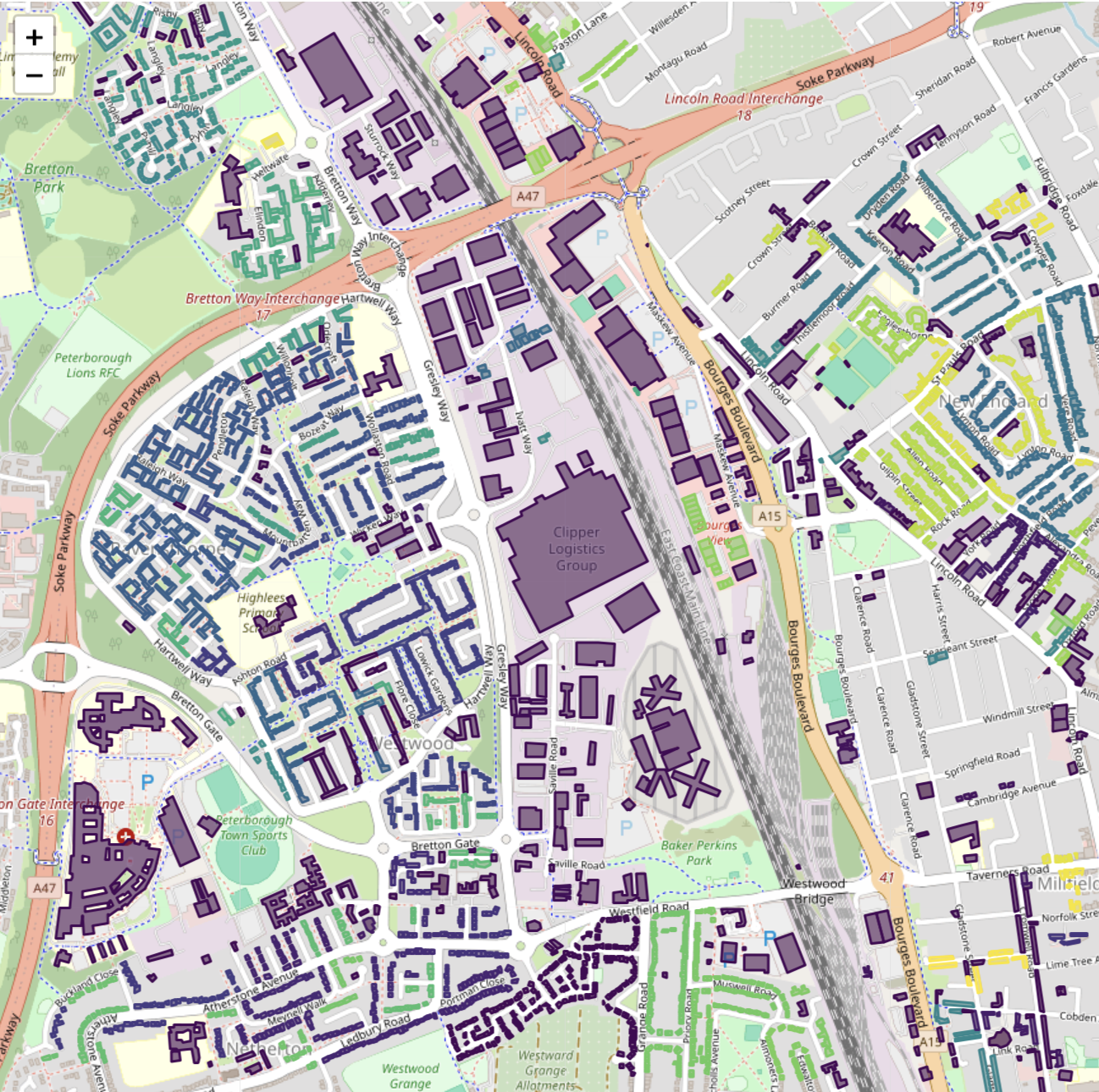 Sklearn clusters using point geometries and the original epsilon plus the median of the buildings’
 minimum_bounding_radius
Adding the median of the buildings’ minimum_bounding_radius to epsilon yields the best match to the clusters found using actual polygons.
A closer inspection of the clusters on a map reveals why they are different:
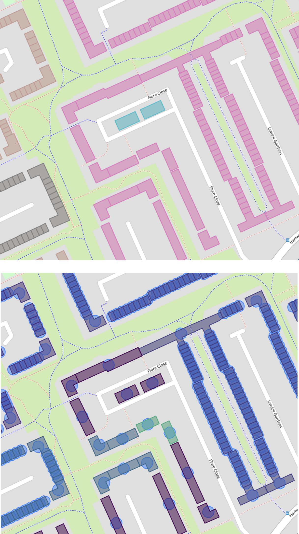
Top: clusters from PostGIS using polygons. Bottom: clusters from Sklearn DBSCAN using minimum-bounding-circle centroids as points and adding the median minimum-bounding-radius to DBSCAN’s epsilon in order to model the buildings as circles (circles are plotted on top of buildings). Elongated building are mis-represented with this approach, and break clusters apart.
Pros and cons of using DBSCAN in PostGIS vs. Python:
Running DBSCAN directly in PostGIS has the advantage of keeping everything within the database:
- no data transfer overhead,
- no need to set up separate environments,
- clustering results are immediately available for further SQL-based processing.
This reduces complexity and improves performance, especially for large geospatial datasets stored in PostgreSQL.
On the other hand, using Python offers more flexibility—you can fine-tune parameters, apply custom distance functions, and even parallelise clustering across data batches if some form of pre-clustering is possible. However, this comes at the cost of increased complexity, particularly around data extraction and preprocessing, such as computing custom distance matrices outside the database.
Conclusion
PostGIS’s ST_ClusterDBSCAN is a powerful, no-fuss solution for clustering real-world geometries—right where your data lives. It handles complex spatial relationships natively, scales well, and avoids the overhead of external tools. If you’re already using PostGIS, there’s no reason not to take full advantage of it for spatial clustering.