Unlocking the Power of Spatial Clustering with DBSCAN

DBSCAN, how it works, different implementations and which ones can handle non-point geometries as inputs?

When working with geospatial data, finding patterns and grouping similar points can unlock valuable insights — whether it’s detecting urban hotspots, mapping wildlife habitats, or analysing customer distribution. One of the most effective clustering algorithms for spatial data is DBSCAN (Density-Based Spatial Clustering of Applications with Noise). Unlike traditional clustering methods like K-means, DBSCAN excels at discovering clusters of arbitrary shape and identifying noise (outliers) in large datasets. See for example the scikit-learn clustering comparison.

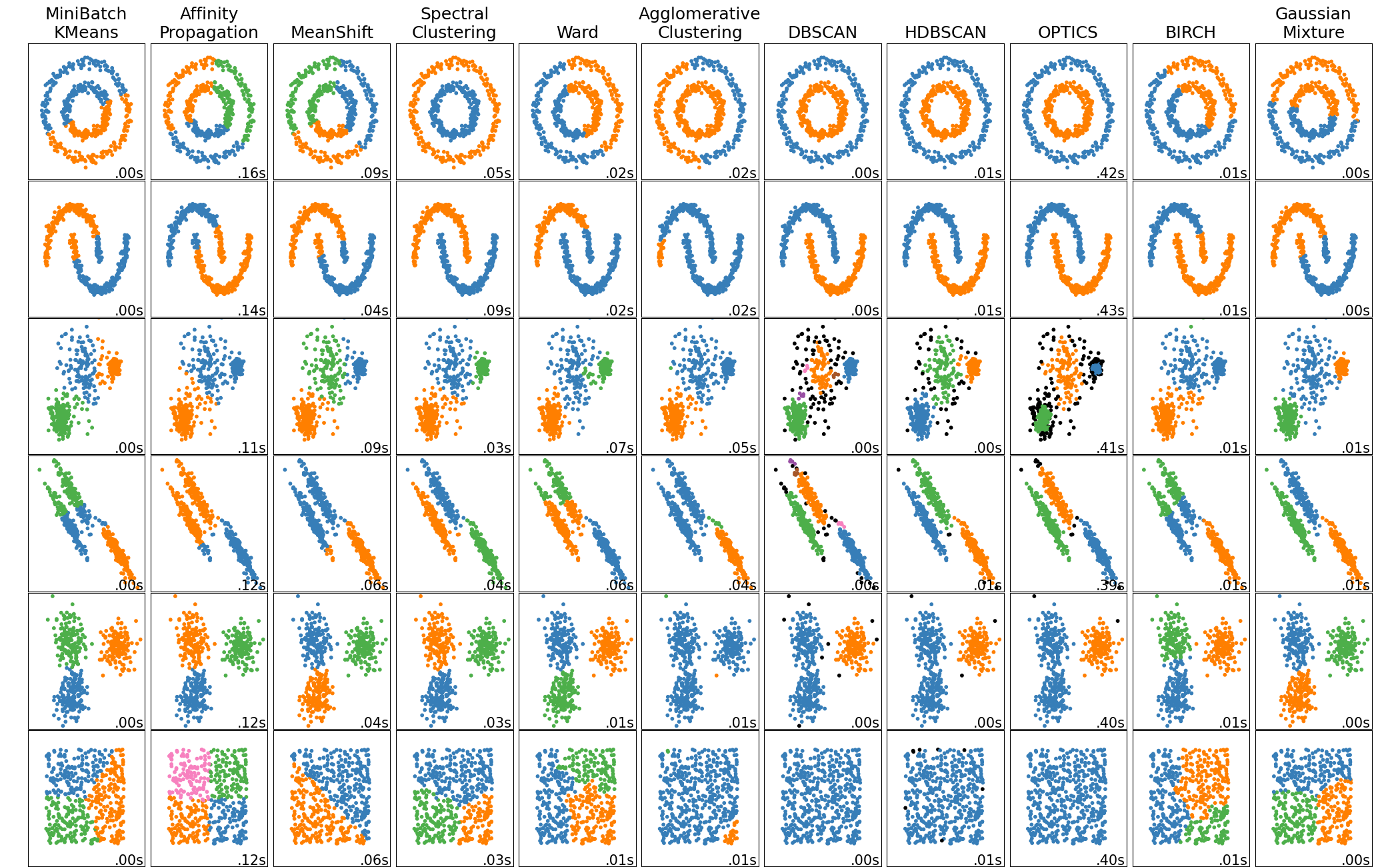Scikit-learn’s clustering comparison. DBSCAN finds arbitrary shapes and allows for outliers.

Understanding DBSCAN: Density-Based Clustering Made Simple

DBSCAN is a powerful clustering algorithm designed to identify groups of data points based on their density. Unlike traditional methods like K-Means, which assume clusters are spherical and require specifying the number of clusters in advance, DBSCAN automatically detects clusters of arbitrary shapes and filters out noise (outliers).

How DBSCAN Works

DBSCAN relies on two key parameters:

• ε (epsilon) – The maximum distance within which points are considered “neighbours.”
• minPts – The minimum number of points required to form a dense region (a cluster).

The algorithm classifies points into three categories:

1. Core Points – Have at least minPts neighbours within a radius of ε.
2. Border Points – Have fewer than minPts neighbours but are close to a core point.
3. Noise (Outliers) – Do not belong to any cluster.

Clusters grow by expanding from core points, connecting neighbouring points that meet the density criteria. If a point does not belong to any dense region, it is labeled as noise.

Why Use DBSCAN?

• Works well with irregularly shaped clusters
• Automatically detects the number of clusters
• Handles noise and outliers effectively
• Performs well with large datasets

However, DBSCAN can struggle with varying densities and high-dimensional data, where choosing the right ε becomes tricky. An extension of DBSCAN that handles density variations is HDBSCAN.

Use Cases

• Geospatial clustering (e.g., identifying urban hotspots)
• Anomaly detection (e.g., fraud detection in transactions)
• Image segmentation
• Social network analysis

By leveraging density-based clustering, DBSCAN offers a flexible and powerful approach to uncovering patterns in complex datasets.

Popular Libraries That Implement DBSCAN

The DBSCAN algorithm is widely used in data science, and multiple libraries across different programming languages provide efficient implementations. Here are some of the most popular ones:

Python

1. scikit-learn (sklearn.cluster.DBSCAN) – A well-optimised, easy-to-use implementation in the popular machine learning library.

from sklearn.cluster import DBSCAN
dbscan = DBSCAN(eps=0.5, min_samples=5).fit(data)

2. HDBSCAN (hdbscan) – A hierarchical, more flexible extension of DBSCAN that automatically selects the best clusters.

import hdbscan
clusterer = hdbscan.HDBSCAN(min_cluster_size=5)
cluster_labels = clusterer.fit_predict(data)

Notice the lack of epsilon parameter? HDBSCAN is basically a DBSCAN implementation for varying epsilon values and therefore only needs the minimum cluster size as single input parameter.

3. cuML (cuml.DBSCAN) – A GPU-accelerated version of DBSCAN for handling large datasets efficiently (part of NVIDIA’s RAPIDS AI framework).

from cuml.cluster import DBSCAN
dbscan = DBSCAN(eps=0.5, min_samples=5)
labels = dbscan.fit_predict(data)

R

4. dbscan (from the dbscan package) – A fast implementation optimized for spatial clustering.

library(dbscan)
result <- dbscan(data, eps = 0.5, minPts = 5)

MATLAB

5. dbscan (from Statistics and Machine Learning Toolbox) – A built-in function for clustering numerical data.

labels = dbscan(data, 0.5, 5);

Julia

6. Clustering.jl (DBSCAN) – A high-performance implementation in Julia.

using Clustering
result = dbscan(data, 0.5, 5)

Apache Spark (for Big Data)

7. MLlib (DBSCAN in Spark MLlib) – Scales DBSCAN to distributed computing environments.

from pyspark.ml.clustering import DBSCAN
dbscan = DBSCAN(eps=0.5, min_samples=5).fit(df)

SQL/PostGIS

8. PostGIS (ST_ClusterDBSCAN) – Implements DBSCAN directly within PostgreSQL, making it great for geospatial clustering.

SELECT 
	id, 
	ST_ClusterDBSCAN(geom, eps := 0.001, minpoints := 5) OVER ()
FROM 
	spatial_data;

These implementations make DBSCAN accessible across various domains, from geospatial analysis to big data clustering and GPU-accelerated machine learning.

Handling Non-Point Geometries with DBSCAN

As already mentioned DBSCAN is good for arbitrarily shaped clusters, but what if the objects we want to cluster also already have a shape, e.g. buildings (polygons) or lines?

Most DBSCAN implementations are optimised for point-based clustering, but some can be adapted to handle non-point geometries (e.g., polygons, lines) by using custom distance metrics, distance/similarity matrix or spatial indexing.

Here’s a breakdown of which implementations support non-point geometries, which require a precomputed distance matrix, and which only support point geometries.

Implementations That Cannot Handle Non-Point Geometries Easily

These implementations do not support non-point geometries or precomputed distances:

• R (dbscan package) No built-in support for non-point data.
• MATLAB (dbscan function) Only works with numerical vectors (points).
• Apache Spark MLlib (DBSCAN) Designed for large-scale point clustering, no support for custom distances.

Implementations That Require a Precomputed Distance Matrix

These libraries only support point data natively, but you can extend them to non-point geometries by manually computing a distance matrix before clustering:

HDBSCAN (hdbscan)

clusterer = hdbscan.HDBSCAN(metric='precomputed')
labels = clusterer.fit_predict(distance_matrix)

scikit-learn (DBSCAN)

from sklearn.cluster import DBSCAN
dbscan = DBSCAN(eps=0.5, min_samples=5, metric='precomputed')
labels = dbscan.fit_predict(distance_matrix)

In both: distance_matrix is a square (n_samples,n_samples) pairwise distance matrix or a scipy sparse array.

cuML (cuml.DBSCAN) Best for: Large-scale clustering on GPU-accelerated systems. If metric is precomputed, X is assumed to be a distance matrix and must be square.

from cuml.cluster import DBSCAN
dbscan = DBSCAN(eps=0.5, min_samples=5, metric='precomputed')
labels = dbscan.fit_predict(X)

Clustering.jl (DBSCAN in Julia) Pass the square distance matrix D and use distances=true keyword argument:

using Clustering
result = dbscan(D, 0.5, 5; distances=true)

Implementations That Can Handle Non-Point Geometries Directly

And now to our absolute winner!

The reason we’ll be focusing on PostGIS (ST_ClusterDBSCAN) in our next article DBSCAN in PostGIS is because it is the only implementation that can process non-point geometries (polygons, lines, etc.), in addition to work directly in the database.

PostGIS (ST_ClusterDBSCAN)

SELECT id, ST_ClusterDBSCAN(geom, eps := 0.001, minpoints := 5) OVER ()
FROM spatial_data;

It is also fast when using spatial indexing and can use different geospatial distances (e.g., great-circle or planar distances) depending on Coordinate Reference System (CRS) and data-type (geometry or geography).

Summary

Library	Supports Non-Point Geometries?	Requires Precomputed Distance Matrix?
PostGIS (ST_ClusterDBSCAN)	✅ Yes (direct support)	❌ No (built-in geospatial distance)
HDBSCAN (hdbscan)	❌ No (points only)	✅ Yes (if using precomputed distances)
scikit-learn (DBSCAN)	❌ No (points only)	✅ Yes (must provide a distance matrix)
cuML (cuml.DBSCAN)	❌ No (points only)	✅ Yes (must provide a distance matrix)
Clustering.jl (DBSCAN)	❌ No (points only)	✅ Yes (must provide a distance matrix)
R (dbscan package)	❌ No	❌ No
MATLAB (dbscan)	❌ No	❌ No
Apache Spark MLlib (DBSCAN)	❌ No	❌ No

Key Takeaways

• Best for non-point geometries?: PostGIS (ST_ClusterDBSCAN) is the best option because it natively handles all spatial data types.

• Need a precomputed distance matrix?: scikit-learn, cuML, HDBSCAN, and Julia can cluster non-point geometries only if you manually compute a distance matrix.

• Not suited for non-point data?: R, MATLAB, and Spark only work with numerical (point) data.

Conclusion

DBSCAN is a powerful tool for uncovering patterns in spatial data, especially when clusters are irregularly shaped or contain noise. While many libraries implement DBSCAN, their ability to handle non-point geometries varies greatly.

PostGIS’s ST_ClusterDBSCAN stands out as the only solution that natively supports complex geometries like polygons and lines — making it ideal for true geospatial clustering directly within the database. In contrast, libraries like scikit-learn, HDBSCAN, cuML, and Clustering.jl can handle such data only if a distance matrix is precomputed.

For simple point data, most implementations will work. But for spatial datasets with richer geometry, PostGIS is the clear choice.