A Simple Geospatial Setup

A streamlined, containerised setup for geospatial data projects using Docker Compose.

By integrating a PostGIS database for geospatial data storage, a GDAL-powered client for data processing, and JupyterLab for interactive analysis, this setup provides a robust and modular solution for geospatial workflows. With persistent data storage, seamless service communication, and custom Dockerfiles, it simplifies tasks like ETL pipelines, database management, and advanced visualization. Whether you’re a GIS professional or a data scientist, this guide offers a scalable and reproducible foundation to enhance your geospatial projects.

The repo can be found here. Here’s the main files in it:

.
├── README.md
├── code
│   └── look_at_data.ipynb
├── compose.yaml
├── dockerfile
├── geo_notebook
│   ├── dockerfile
│   └── requirements.txt
└── makefile

The compose.yaml file is a Docker Compose configuration file that defines and manages multiple services in a containerized environment.

The geo_notebook and client service are referred to in the compose.yaml and built from two custom Dockerfiles (geo_notebook/dockerfile and dockerfile, respectively), we’ll look into them in more detail now.

Get it up and running

For the impatient reader here’s how to get the services up and running or checkout the quick giude:

Prerequisites

Docker installed: Ensure Docker is installed on your system. Docker is available for Windows, macOS, and Linux. Installation instructions can be found on the Docker website.
.env file You can create an .env file at the root of the repo to set the following environment variables

# postgres credentials and DB name to use
POSTGRES_USER=pg
POSTGRES_PASSWORD=pg
POSTGRES_DB=pg
# the token for jupyter and jupyter port number on your host machine
JUPYTER_TOKEN=mytoken
JUPYTER_PORT=8889

Or add export them to your shell before running docker compose up. See here for more info on passing environment variables to docker compose as well as precedence and interpolation of variables.

Run the Services

For convenience a makefile is added to the repository so you can (re)start all services and get the link to the Jupyter server with one command:

make all

or just run

docker compose up -d

if you only want a PostGIS and the jupyter server run:

docker compose up -d geo_notebook

Using JUPYTER_TOKEN=mytoken and JUPYTER_PORT=8889 the Jupyter server should be accessible at: http://127.0.0.1:8889/?token=mytoken .

We’ll now run step by step through the docker-compose.yaml file and the dockerfies making uo the db, client and geo_notebook services.

Understanding the compose.yaml File

The compose.yaml file is a configuration file for Docker Compose, a tool used to define and manage multi-container Docker applications. This file specifies the services, networks, and volumes required to run the application.

compose.yaml:

version: '3.8'
 
services:
  db:
    image: postgis/postgis:latest
    environment:
      POSTGRES_USER: ${POSTGRES_USER}
      POSTGRES_PASSWORD: ${POSTGRES_PASSWORD}
      POSTGRES_DB: ${POSTGRES_DB}
    ports:
      - ${EXTERNAL_IP:-127.0.0.1}:5432:5432
    volumes:
      - ./data/postgis_data:/var/lib/postgresql/data:rw
    networks:
      - net
  client:
    build:
        dockerfile: dockerfile
        context: .
        args:
            - no-cache
    tty: true
    volumes:
      - './data/raw:/data/raw:rw'
    environment:
      POSTGRES_USER: ${POSTGRES_USER}
      POSTGRES_PASSWORD: ${POSTGRES_PASSWORD}
      POSTGRES_DB: ${POSTGRES_DB}
      PGHOST: db
    networks:
      - net
    depends_on:
      - db
  geo_notebook:
    build:
      dockerfile: dockerfile
      context: ./geo_notebook
    environment:
      POSTGRES_USER: ${POSTGRES_USER}
      POSTGRES_PASSWORD: ${POSTGRES_PASSWORD}
      POSTGRES_DB: ${POSTGRES_DB}
      PGHOST: db
      JUPYTER_TOKEN: ${JUPYTER_TOKEN}
    ports:
      - ${JUPYTER_PORT:-8889}:8888
    volumes:
      - './code:/code:rw'
      - './data/raw:/data/raw:rw'
    networks:
      - net
    depends_on:
      - db
  
networks:
  net:
    driver: bridge

The version specifies the Docker Compose file format. Here’s a breakdown of what the file does.

Services

The services section defines the containers that make up the application. In this file, there are three services: db, client, and geo_notebook.

`db` Service

db:
  image: postgis/postgis:latest
  environment:
    POSTGRES_USER: ${POSTGRES_USER}
    POSTGRES_PASSWORD: ${POSTGRES_PASSWORD}
    POSTGRES_DB: ${POSTGRES_DB}
  ports:
    - ${EXTERNAL_IP:-127.0.0.1}:5432:5432
  volumes:
    - ./data/postgis_data:/var/lib/postgresql/data:rw
  networks:
    - net

Image: Uses the postgis/postgis:latest image, which is a PostgreSQL database with PostGIS extensions for geospatial data.
Environment Variables: Configures the database using variables (POSTGRES_USER, POSTGRES_PASSWORD, POSTGRES_DB) that are defined in a .env file or the shell environment.
Ports: Maps the database’s port 5432 to the host machine. If EXTERNAL_IP is not set, it defaults to 127.0.0.1.
Volumes: Mounts a local directory (./data/postgis_data) to persist database data.
Networks: Connects the service to the net network.

`client` Service

client:
  build:
    dockerfile: dockerfile
    context: .
    args:
      - no-cache
  tty: true
  volumes:
    - './data/raw:/data/raw:rw'
  environment:
    POSTGRES_USER: ${POSTGRES_USER}
    POSTGRES_PASSWORD: ${POSTGRES_PASSWORD}
    POSTGRES_DB: ${POSTGRES_DB}
    PGHOST: db
  networks:
    - net
  depends_on:
    - db

Build: Builds the container from a dockerfile in the current directory (.). The no-cache argument ensures a fresh build.
TTY: Keeps the container running interactively.
Volumes: Mounts a local directory (./data/raw) for shared data.
Environment Variables: Configures the service to connect to the db service using the same database credentials.
Networks: Connects to the net network.
Depends On: Ensures the db service starts before this service.

Note: the database service db is also the host-name of the database within the docker-compose network. If you want to access the DB from a DB tool like DBbeaver or a Python script running locally but outside the docker network, the host is localhost (or 127.0.0.1 and port the mapped port in db service:ports.*

geo_notebook Service

geo_notebook:
  build:
    dockerfile: dockerfile
    context: ./geo_notebook
  environment:
    POSTGRES_USER: ${POSTGRES_USER}
    POSTGRES_PASSWORD: ${POSTGRES_PASSWORD}
    POSTGRES_DB: ${POSTGRES_DB}
    PGHOST: db
    JUPYTER_TOKEN: ${JUPYTER_TOKEN}
  ports:
    - ${JUPYTER_PORT:-8889}:8888
  volumes:
    - './code:/code:rw'
    - './data/raw:/data/raw:rw'
  networks:
    - net
  depends_on:
    - db

Build: Builds the container from a Dockerfile in the geo_notebook directory.
Environment Variables: Configures the service to connect to the db service and sets the JupyterLab token (JUPYTER_TOKEN).
Ports: Maps the Jupyter default port 8888 to the host machine. If JUPYTER_PORT is not set, it defaults to 8889 to not interfere with any existing Jupyter server.
Volumes: Mounts local directories for code (./code) and raw data (./data/raw).
Networks: Connects to the net network.
Depends On: Ensures the db service starts before this service.

Networks

networks:
  net:
    driver: bridge

Defines a custom network named net using the bridge driver. This allows the services to communicate with each other.

Understanding the Dockerfiles in the Project

Now we’ll walk through the Dockerfiles the geo_notebook and client services are built from.

Dockerfile for geo_notebook

This Dockerfile defines the environment for the geo_notebook service.

FROM quay.io/jupyter/minimal-notebook:python-3.12
ENV PYTHONUNBUFFERED 1
COPY ./requirements.txt requirements.txt
RUN pip install -Ur requirements.txt
RUN mkdir code
WORKDIR /code

Base Image: Starts from the quay.io/jupyter/minimal-notebook:python-3.12 image, which provides a minimal Jupyter environment with Python 3.12 pre-installed.

Environment Configuration: Sets the PYTHONUNBUFFERED environment variable to 1, ensuring that Python output is immediately flushed to the console (useful for debugging).

Installing Dependencies: Copies a requirements.txt file into the container and installs the Python dependencies listed in it using pip.

Directory Setup:

Creates a code directory inside the container (this will also be our volume on the host machine so we persist our notebooks and they don’t get lost when containers are stopped).
Sets the working directory to code, where the container will start executing commands.

Dockerfile for a GDAL Client

GDAL (Geospatial Data Abstraction Library) is widely used for geospatial data processing, and this setup is tailored for geospatial workflows. This Dockerfile defines a custom Docker image based on the GDAL image.

This setup is particularly useful for:

Running geospatial queries on PostgreSQL/PostGIS databases.
Manipulating geospatial data stored in SQLite databases.
Converting raw OpenStreeMap data to GeoJson.
Using GDAL tools for raster and vector data processing.
Importing and exporting data to and from PostGIS

# Use the latest Ubuntu-based full GDAL image from the GitHub Container Registry
FROM ghcr.io/osgeo/gdal:ubuntu-full-latest
 
# Set the environment variable to suppress interactive prompts during package installation
ENV DEBIAN_FRONTEND=noninteractive
 
# Update the package list and install PostgreSQL client and SQLite3
RUN set -x \  
    && apt-get update \
    && apt-get install -y \
        postgresql-client \ 
        sqlite3 \
        npm 
# Install the  Node.js osmtogeojson package for converting osm data to geojson
 
RUN npm install -g osmtogeojson

This Dockerfile is designed to create a containerised environment for geospatial data processing. By starting with the GDAL image and adding database clients, it provides a versatile setup for working with geospatial data stored in PostgreSQL (with PostGIS extensions) or SQLite and npm in order to then install the osmtogeojson package.

Here’s a breakdown of what each line does:

The base image ghcr.io/osgeo/gdal:ubuntu-full-latest is a full-featured GDAL image based on Ubuntu that includes GDAL and its dependencies, making it suitable for geospatial data processing tasks such as raster and vector data manipulation. For example it includes the powerful ogr2ogr library that we’ll cover separately. REF: geo-imports ARTICLE

ENV DEBIAN_FRONTEND=noninteractive

Sets the DEBIAN_FRONTEND environment variable to noninteractive. This ensures that when apt-get commands are run, they do not prompt for user input, which is essential for automated builds.

Installing Additional Tools

RUN set -x \
    && apt-get update \
    && apt-get install -y \
        postgresql-client \
        sqlite3\
        npm
 
RUN npm install -g osmtogeojson

set -x: Enables debugging by printing each command before it is executed.
apt-get update: Updates the package lists to ensure the latest versions of packages are available.
apt-get install -y: Installs the following tools:
- postgresql-client: A command-line client for PostgreSQL, allowing the container to interact with PostgreSQL databases (e.g., running SQL commands or managing databases).
- sqlite3: A lightweight command-line tool for interacting with SQLite databases, useful for local or small-scale geospatial data storage.
- npm: the default package manager for Node.js, used to install, manage, and share JavaScript packages and dependencies.

RUN npm install -g osmtogeojson: installs the package osmtogeojson globally (-g flag). osmtogeojson is a small Node.js library (and CLI tool) that converts OpenStreetMap JSON data (from Overpass API, for example) into standard GeoJSON format, which is easy to use with GIS software like QGIS, Leaflet, Mapbox or ogr2ogr to import to PostGIS.

How It All Works Together

Database Setup: The db service provides a PostgreSQL database with PostGIS extensions for geospatial data storage and querying.
Client Service: The client is a lightweight yet powerful environment for geospatial workflows. It combines the capabilities of GDAL with database clients, making it suitable for geospatial data extraction, transformation, and loading (ETL), as well as database management and analysis.
JypterLab: The geo_notebook service provides a JypterLab environment for geospatial data analysis and visualization. It connects to the database (db) for querying and processing geospatial data.
Shared Network: All services communicate over the net network, allowing seamless interaction between the database, client, and notebooks.
Persistent Data: Data and code is stored persistently on the host machine using volume mounts, ensuring that database and raw data are not lost when containers are stopped.

Summary

This setup is a powerful, modular solution for geospatial data projects. It combines the strengths of PostGIS for geospatial data storage, GDAL for data processing, and JypterLab for interactive analysis.

By leveraging Docker Compose, the environment is easy to manage, scalable, and ensures reproducibility across different systems. Whether you’re working on geospatial ETL pipelines, database management, or advanced data visualisation, this setup provides a robust foundation to streamline your workflows.

PostGIS, GDAL and Jupyter together in Action

This second part is a quick walk through two ways of pulling data from OpenStreetMap and pushing it to PostGIS. One requires the osmtogeojson dependency the other doesn’t.

All the following commands are run within the client container so run

docker compose run client bash

first in order to continue working from within the client’s command line.

Getting Data from OSM via cURL from Client to PostGIS

Option 1: Download as OSM style json and use `osmtogeojson` to convert to GeoJson

First download all cafes in Paris into OSM style .json:

curl -X GET "https://overpass-api.de/api/interpreter" \
--data-urlencode 'data=[out:json];area[name="Paris"]->.searchArea;node["amenity"="cafe"](area.searchArea)(48.52,1.73,49.22,3.00);out body;' \
-o data/raw/paris_cafes.json

since org2ogr doesn’t have a driver for OSM’s .json format you need to convert it to .geojson:

osmtogeojson data/raw/paris_cafes.json > data/raw/paris_cafes.geojson

Now you can use ogr2ogr to push the content of the GeoJson into a new table called paris_cafes_osm2gj.

ogr2ogr -f "PostgreSQL" \
    PG:"host=$PGHOST user=$POSTGRES_USER dbname=$POSTGRES_DB password=$POSTGRES_PASSWORD" \
    "data/raw/paris_cafes.geojson" \
    -nln "paris_cafes_osm2gj" \
    -overwrite \
    -lco GEOMETRY_NAME=geom \
    -lco FID=gid \
    -lco PRECISION=NO \
    -progress \
    -skipfailures

Pros:

flexible: all geometry types in one go regardless of what is in the output of the OSM query.
handles attributes and tags properly by turning them into json fields and each tag becomes a column in PostgreSQL Cons:
dependencies: needs npm and osmtogeojson installed.

Option 2: Download as OSM XML use `ogr2ogr` to write directly to PostGIS

This alternative pulls the data in the .osm format for which ogr2ogr has a driver.

The query looks very similar to the one above, but instead of pulling OSM style json it’s pulling an .osm file.

curl -X GET "https://overpass-api.de/api/interpreter" \
--data-urlencode 'data=area[name="Paris"]->.searchArea;node["amenity"="cafe"](area.searchArea)(48.52,1.73,49.22,3.00);out;' \
-o data/raw/paris_cafes.osm

ogr2ogr has a driver to work with this format, however it has strict typing and you have to pick which geometry type we want to push to the DB:

ogr2ogr -f "PostgreSQL" \
    PG:"host=$PGHOST user=$POSTGRES_USER dbname=$POSTGRES_DB password=$POSTGRES_PASSWORD" \
    "data/raw/paris_cafes.osm" \
    points\
    -nln "paris_cafes" \
    -overwrite \
    -lco GEOMETRY_NAME=geom \
    -lco FID=gid \
    -lco PRECISION=NO \
    -progress \
    -skipfailures

Notice the points argument? You would need to repeat this command as an -append rather than -overwrite command, and add all possible other geometry-types: (lines, multi-linestrings, multi-polygons etc.)

docker compose run client \
ogr2ogr -f "PostgreSQL" \
    PG:"host=$PGHOST user=$POSTGRES_USER dbname=$POSTGRES_DB password=$POSTGRES_PASSWORD" \
    "data/raw/paris_cafes.osm" \
    lines\
    -nln "paris_cafes" \
    -append
    ...

For more on this, see https://gis.stackexchange.com/questions/339075/convert-large-osm-files-to-geojson

Pros: No extra dependencies. Cons:

separate handling of points, lines, multilinestrings, etc
tags get placed into a text column e.g. "addr:city"=>"Paris","addr:housenumber"=>"93",..., "opening_hours"=>"Mo-Su 08:00-02:00","wikidata"=>"Q17305044" and would require extra processing to be queried.

Query and Plot in a Notebook

Now it’s time to go and see the data! You should have a Jupyter server runnning at: http://127.0.0.1:${JUPYTER_PORT}/?token=${JUPYTER_TOKEN} So with the default environment variables that’s http://127.0.0.1:8889/?token=mytoken .

You can also use:

make jupyter-url

to print the link to the Jupyter server.

The notebook look_at_data.ipynb sets up the connection to the DB so you can use it with Pandas or Geopandas or whatever you prefer.

import os
from sqlalchemy import create_engine
pg_user = os.getenv('POSTGRES_USER')
pg_pw = os.getenv('POSTGRES_PASSWORD')
pg_db = os.getenv('POSTGRES_DB')
port = 5432
host = 'db' # service name of database within docker network
 
engine = create_engine(f"postgresql+psycopg2://{pg_user}:{pg_pw}@{host}:{port}/{pg_db}")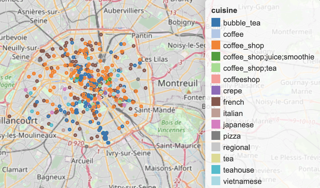

Folium map of cafes with the top 15 types of cuisines in in Paris.

Wrapping Up: A Modular Geospatial Playground in Docker

In this article, we explored how to set up a clean, containerised geospatial development environment using Docker Compose. By combining the strengths of PostGIS, GDAL, and JupyterLab, you’ve got yourself a powerful little toolkit for geospatial workflows — one that handles everything from data extraction to visualisation.

This setup isn’t just another “hello world” — it’s designed to mirror the kind of real-world, multi-stage pipelines you’d find in production:

PostGIS for storing and querying spatial data,
GDAL tools and a custom client for data wrangling and transformation,
JupyterLab for the exploration and visualisation phase.

Whether you’re building ETL pipelines, automating Geodata imports, or just experimenting with OpenStreetMap data, this environment lowers the friction and makes your workflow reproducible and easy to share. By keeping services loosely coupled, you can swap, extend, or scale components as your project evolves.

Conslusion

A well-structured development environment is like a good map — it doesn’t just show you where you are, it shows you how to get where you’re going.

This Docker-based setup brings together some of the most reliable open-source tools in geospatial analysis and wraps them in a developer-friendly package. No more dependency headaches, no more “works on my machine” — just a clean, modular setup for geospatial data science.

If you’re ready to dive in, check out the full repository here and start exploring the world of spatial data the way it’s meant to be: interactive, efficient, and fun.

Dr. Riccardo Scott

Explorer

A Simple Geospatial Setup

Get it up and running

Prerequisites

Run the Services

Understanding the compose.yaml File

Services

`db` Service

`client` Service

geo_notebook Service

Networks

Understanding the Dockerfiles in the Project

Dockerfile for geo_notebook

Dockerfile for a GDAL Client

How It All Works Together

Summary

PostGIS, GDAL and Jupyter together in Action

Getting Data from OSM via cURL from Client to PostGIS

Option 1: Download as OSM style json and use `osmtogeojson` to convert to GeoJson

Option 2: Download as OSM XML use `ogr2ogr` to write directly to PostGIS

Query and Plot in a Notebook

Wrapping Up: A Modular Geospatial Playground in Docker

Conslusion

Graph View

Table of Contents

Backlinks

Dr. Riccardo Scott

Explorer

A Simple Geospatial Setup

Get it up and running

Prerequisites

Run the Services

Understanding the compose.yaml File

Services

db Service

client Service

geo_notebook Service

Networks

Understanding the Dockerfiles in the Project

Dockerfile for geo_notebook

Dockerfile for a GDAL Client

How It All Works Together

Summary

PostGIS, GDAL and Jupyter together in Action

Getting Data from OSM via cURL from Client to PostGIS

Option 1: Download as OSM style json and use osmtogeojson to convert to GeoJson

Option 2: Download as OSM XML use ogr2ogr to write directly to PostGIS

Query and Plot in a Notebook

Wrapping Up: A Modular Geospatial Playground in Docker

Conslusion

Graph View

Table of Contents

Backlinks

`db` Service

`client` Service

Option 1: Download as OSM style json and use `osmtogeojson` to convert to GeoJson

Option 2: Download as OSM XML use `ogr2ogr` to write directly to PostGIS